RelGNN: reading a database as a set of atomic routes
Your company's database is secretly a graph. A graph neural network can walk it, but the edges are only foreign-key plumbing, and walking them naively makes the network hear the plumbing louder than the signal. RelGNN's fix is a structure so small the authors call it atomic. This is the whole argument, built from scratch.
I worked through this by rebuilding every idea in it from scratch. That's my test for whether I actually understood something. Everything runs on one toy I'll call TinyGrid: a miniature Formula One database. Here it is in full: five tables, two rows each. Keep this picture; every idea in the paper lands somewhere on it.
| driver_id | name |
|---|---|
| hamilton | Lewis Hamilton |
| verstappen | Max Verstappen |
| race_id | name |
|---|---|
| monaco | Monaco GP |
| silverstone | British GP |
| constructor_id | name |
|---|---|
| mercedes | Mercedes |
| redbull | Red Bull |
| standing_id | race_id | driver_id | points |
|---|---|---|---|
| s1 | monaco | hamilton | 18 |
| s2 | silverstone | hamilton | 25 |
| result_id | race_id | driver_id | constructor_id | position |
|---|---|---|---|---|
| r1 | monaco | hamilton | mercedes | 2 |
| r2 | silverstone | verstappen | redbull | 1 |
bold = primary key (the row's unique name-tag) shaded ↗ = foreign key (a pointer at another table's name-tag)
Look at the last two tables and you can already see the shape of the whole problem. drivers, races and constructors are the things you actually care about, and they hold no pointers at all. Every connection between them has to run through standings or results, tables that exist mostly to hold pointers. Count those pointers and you've classified the table: two makes a bridge, three or more makes a hub. That count is the entire taxonomy, and chapter one is about what it does to a neural network.
The question we keep asking throughout: will Hamilton finish in the top three of his next race? The only things you need to bring: you know what a vector is, and you believe a neural network is a trainable function, a box with knobs. No graph theory, no databases, no attention. We build all of it here.
Chapter one
Your database is a graph, and message passing is going blind
Tables are already a graph
Every row in a table has one column that is its unique name-tag, its primary key. Hamilton's driver-id, Monaco's race-id. A row can also store a pointer to another table's name-tag, and that pointer is a foreign key. Look back at the results table: its race_id column holds the value monaco, which is a race's primary key. That's all a foreign key is: this row relates to that row.
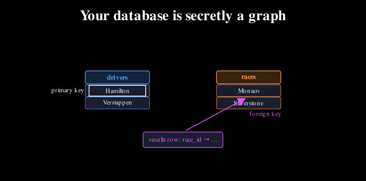
And there's the secret. A foreign key is an edge. Make every row a dot, draw a line for every foreign-key pointer, and the whole database becomes one graph. Rows are nodes; each table becomes a node-type. The field calls the result a relational entity graph, and running neural nets on it relational deep learning.
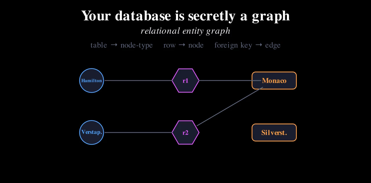
One thing this picture insists on: time. Every event carries a timestamp, and when we predict Hamilton's next race we may only use rows from before that race. Peeking at the future is cheating (the field calls it leakage) and it shapes how the benchmark in chapter three is split.
The catch: these edges carry no verb
So hand the graph to a GNN and go home? Not quite, and the subtlety here is what the whole paper hangs on.
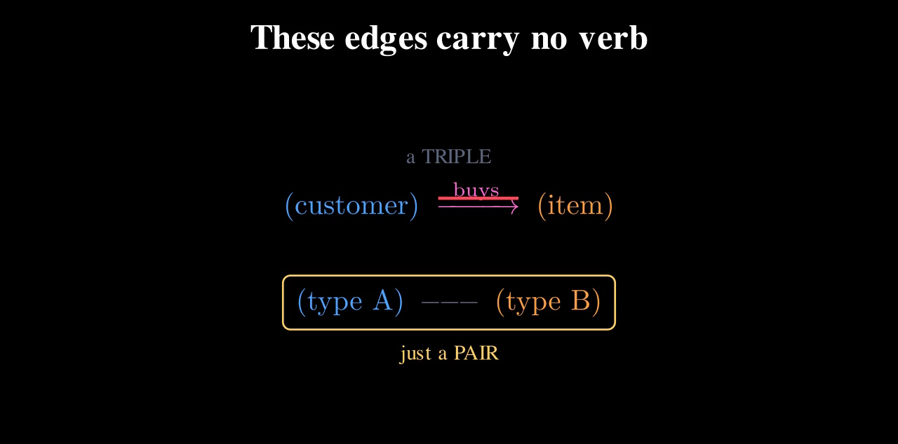
In most graphs an edge carries a meaning. In a social graph an edge says follows, or is friends with. The edge is a relationship, a little verb. Graph networks were designed assuming every edge is a fact like that. Now look at ours. Take the line joining Hamilton to one of his results rows. What verb is on that edge? There isn't one. It only says "this foreign key points here."
That flips the smallest unit of the graph. In a verb-graph the atom is a triple: subject, verb, object; customer buys item. With no verb in the middle, the atom collapses to a pair: this type of thing, linked to that type of thing. Hold onto that word. The entire method is built to respect it.
Bridges and hubs: just count the foreign keys
Here's the squeeze. A foreign key points at exactly one row. So how do you say "one driver runs in many races, and one race holds many drivers"? You might think: give the driver row a column for each race. But a column holds one value per row, and a driver enters dozens of races, and you can't keep bolting on columns. A single pointer cannot express many-to-many.
The database's move is to insert a middle table. To connect drivers and races it builds a standings table, where each row points to exactly one driver and one race. These middle tables are called junction tables, and they are where everything downstream gets tricky.
So sort every table by one number: how many foreign keys it carries. Count the shaded columns in TinyGrid above and you get the whole taxonomy:
- 0 or 1: an ordinary table. drivers, races, constructors: no pointers at all.
- exactly 2: a bridge. It bridges two other types. standings: race_id and driver_id.
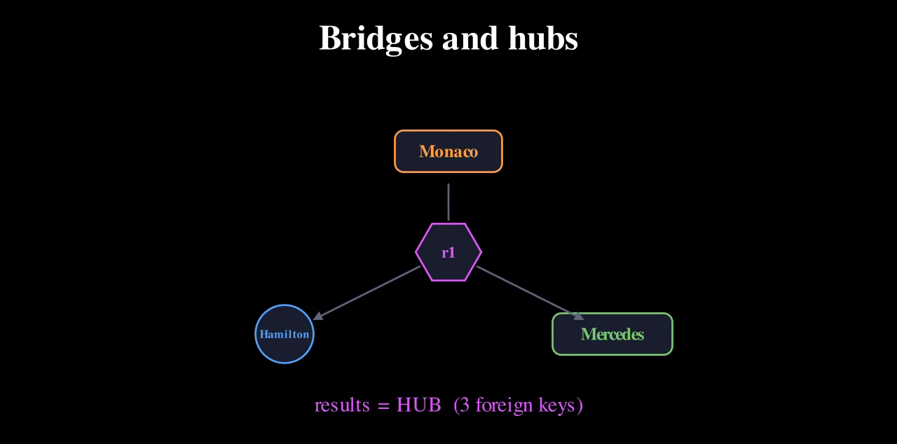
- 3 or more: a hub. It sits at the centre of a star. results: race_id, driver_id and constructor_id.
Message passing, and exactly where it breaks
How does a graph network use a graph? One rule, repeated: each round, every node looks at its neighbours, averages what they hold, and mixes that into itself.
h_v ← avg( h_v , { h_u : u ∈ N(v) } ) real GNN: h_v ← ReLU( W · [ h_v ‖ mean_u h_u ] ) (same wiring, different numbers)
I'll use plain averages so the arithmetic is naked. A real network multiplies by a weight matrix and squashes with a nonlinearity, but that changes only the numbers, not who hears whom. And the wiring is where the whole story lives. One round is one hop: after two rounds a node has heard its neighbours' neighbours.
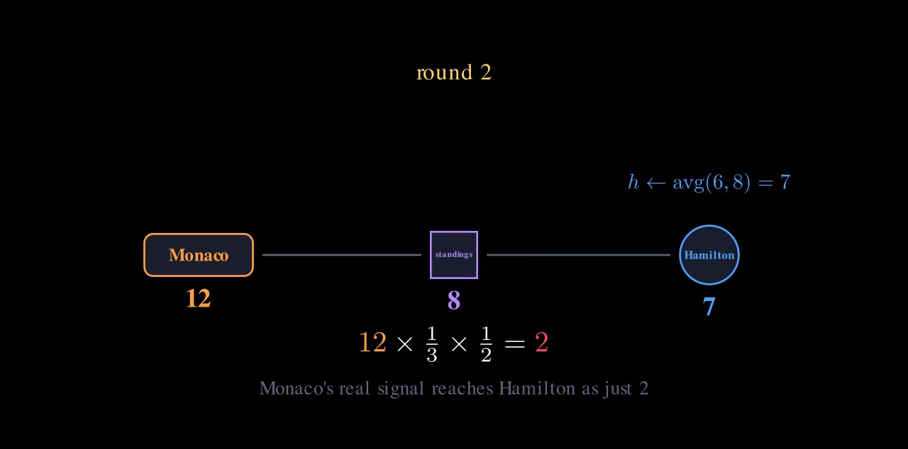
Now watch it fail on the bridge. We want race information to reach the driver: Monaco should inform Hamilton. But they aren't neighbours; the standings router sits between them. Put naked numbers on the three nodes: Monaco 12 (how demanding the track is), Hamilton 9, and the router standings 3. Not empty. Just small.
round 1: standings = avg(3, 12, 9) = 8 Hamilton = avg(9, 3) = 6 Monaco = avg(12, 3) = 7.5 round 2: Hamilton = avg(6, 8) = 7
Failure one: redundancy. A third of that 8 is Hamilton's own 9. Hamilton's information walked into the router in round one, and in round two Hamilton reads the router back. Part of what Hamilton "learns" is its own echo, dressed up as news.
Failure two: imbalance. Of Hamilton's final 7, how much is really Monaco, the node we actually cared about? Monaco's 12 had to survive two averagings: one third when it entered the router, then one half when Hamilton read the router.
You might object that standings had some content too, so maybe that's fine. So stop trusting the specific numbers and ask what the wiring does no matter what you plug in. Break Hamilton's final value into where it came from:
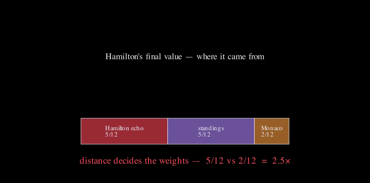
Which should the driver weight more: the router that's mostly a connector, or the race that holds the real signal? The race. Which does the wiring weight more? The router. It has the priorities backwards, and this isn't one network misbehaving: it's what two-hop message passing does to every bridge and every hub in the database. Redundant and imbalanced. That's the villain.
Try these before chapter two
- A tiny school database: students, courses, and an enrolments table where each row links one student to one course. Draw it as a graph. Which table is the bridge?
- Some table carries four foreign keys. Bridge or hub, and what shape does its node make?
- Design question. If you could send Monaco's information straight to Hamilton in a single hop, skipping the router detour, what would you fold in along the way, so you don't throw away what the standings row legitimately knows?
Chapter two
Atomic routes and composite message passing
Answers first. Enrolments has two foreign keys, so it's the bridge. Four foreign keys sits at the centre of a four-armed star: a hub. And question three is the whole chapter: the honest answer is fold the router into the message. Carry the race and the standings row together, in one step, straight to the driver.
The definition
An atomic route is the shortest honest path that lets a source talk to a destination in a single hop. Two cases, and they're just the bridge and hub we already met:
- Single foreign key. The table points at exactly one other table, so the route is that edge, taken both ways.
- Several foreign keys (a bridge or hub). The route threads through it: source → middle → destination.
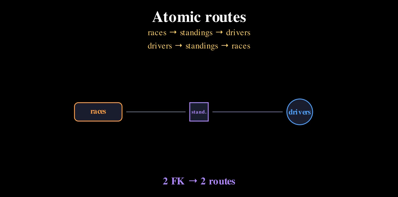
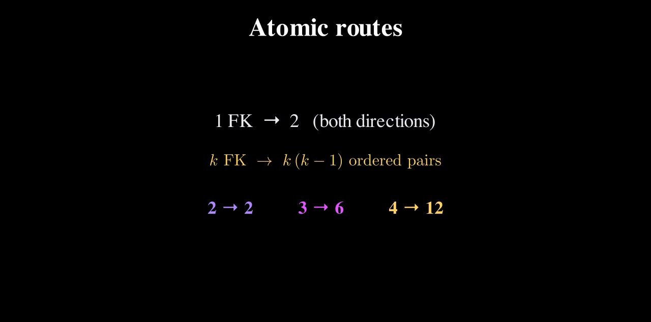
The hub results has three foreign keys: races, drivers, constructors. Same rule: pick a source, pick a different destination, thread through the middle. Three things taken two at a time, in order: six routes. Which gives the rule worth bottling:
Two things make this quietly powerful. First, the routes are derived, not designed. People have hand-built paths through graphs for years; they're called meta-paths. But that needs a domain expert, the paths differ for every database, and whatever the expert forgets, the model never sees. Atomic routes fall out of the foreign keys for free, on any schema, including one nobody has seen.
Second, they're computed on the schema (the handful of table types) not on the rows. A database can have a hundred million drivers and still have a few tables. The route list stays tiny no matter how big the data grows.
Composite message passing
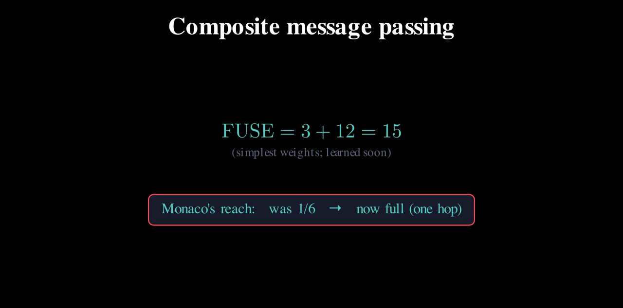
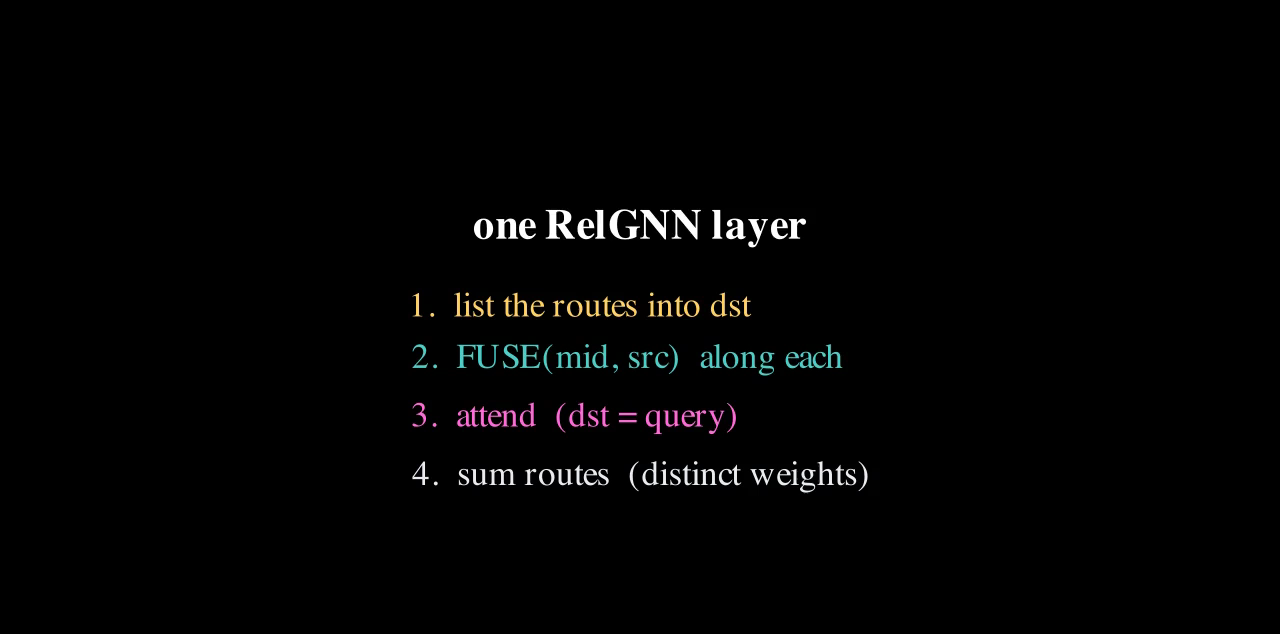
We have the routes. What do we send along them? Don't crawl. For the driver, look along each atomic route at once, and in a single step combine the middle and the source into one message, then let the driver take it in.
eq 3: h_dst ← AGGR( h_dst , { FUSE( h_mid , h_src ) : each route } )
Note carefully what's inside the fused message: the middle and the source. Not the destination.
Two objections are worth voicing, because they're the ones I had.
Doesn't the driver still use its own value? Yes, and it should. A node keeping its own information is healthy, and you'll see it kept as a clean, direct self-term in a moment. What we killed is different: the driver's value being laundered through the router and handed back as if it were outside news. Keeping your own value is fine. Hearing it echoed back disguised as news is the redundancy, and it's gone.
The router's 3 is still in the message, isn't it still over-weighted? The disease was never that the router was present; it was that the source was starved, choked down to a sixth. Give the source its full one-hop weight and the imbalance is cured directly. And if the router's content turns out to be useless, the next ingredient can simply turn its weight down.
Filling in the two blanks
Equation 3 is a template: it says fuse, then aggregate, but not how. RelGNN fills both.
eq 4 FUSE = W1 · h_mid + W2 · h_src (a learnable weighted sum) eq 6 single-FK route: no middle, so the message is just h_src eq 7 h_dst = W_proj · h_dst + Σ over routes m_route (each route its own weights)
FUSE is easy: along a route there are only ever two vectors to blend: one middle and its one source, because a foreign key points to exactly one row. Two vectors, so a learnable weighted sum suffices.
AGGR is where the driver gets to choose. Hamilton isn't on one route: he hears the race through the standings bridge, the race again through the results hub, and his constructor through that same hub. Three fused messages arriving at once. How should he weigh them? That question has a famous answer, attention, and it's four small steps:
- The driver forms a query, each message forms a key. Neither is the raw vector: each is passed through its own small learnable matrix. Those matrices are what training tunes: they're how the model learns what "relevant" means.
- Score each message by how well its key lines up with the query, a dot product.
- Softmax the scores into weights: raise e to each, divide by the total. Positive, summing to one.
- The answer is those weights times the messages themselves, the values.
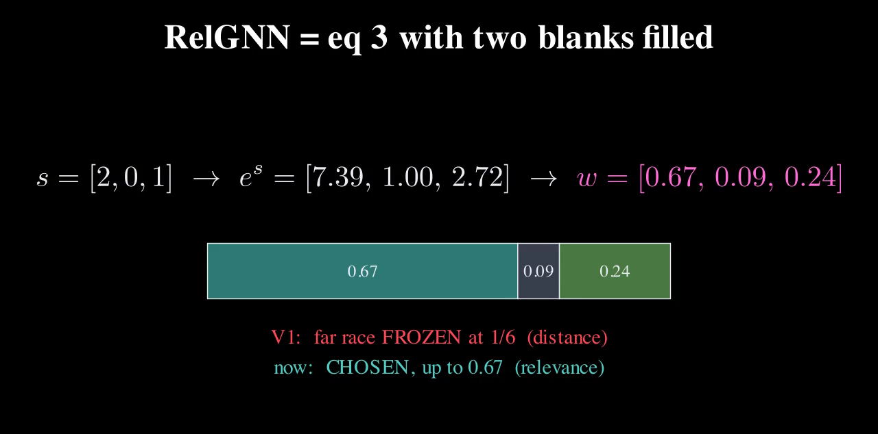
Equation 7 adds one safeguard that's easy to skim past: every route gets its own weight matrices. The race through the bridge and the race through the hub are learned separately, so the model can trust one and distrust the other, and the two never blur into one mush.
Try these before chapter three
- By hand: W1 = I, W2 = 2I, h_mid = [1,3], h_src = [2,1]. What is W1·h_mid + W2·h_src?
- How many atomic routes does a table with four foreign keys create?
- Place a bet. RelGNN has two new ideas: the atomic routes, and the attention on top. Which one actually earns the accuracy? Write it down now.
Chapter three
One layer by hand, and does it hold up?
Answers: the fuse is [1,3] + [4,2] = [5,5]. Four keys give 4 × 3 = 12 routes. The bet stays open until the ablation below, and the result surprised me.
One full update, every number visible
Two rules of the game. We use 2-D embeddings so a vector fits on a line, and we take every weight matrix to be the identity, so FUSE becomes plain addition and the projections pass values through. Real RelGNN learns these; setting them to identity mostly changes how sharply the attention concentrates, not the steps.
Hamilton starts at h = [1, 0] route: races → standings → drivers, arriving twice A: Monaco [2,0] via s1 [0,1] B: Silverstone [0,2] via s2 [1,0]
![Step one, FUSE: fuse A equals [0,1] plus [2,0] equals [2,1]; fuse B equals [1,0] plus [0,2] equals [1,2].](../assets/relgnn/11-walk-fuse.png)
Step 2: score. Hamilton's query is his own vector, [1,0]. Score each fused message by the dot product with the query, divided by the square root of the dimension. That's the scaled in scaled dot-product attention, and it's there so longer vectors don't blow the scores up.
q·[2,1] = 2 → 2 / √2 = 1.41 q·[1,2] = 1 → 1 / √2 = 0.71
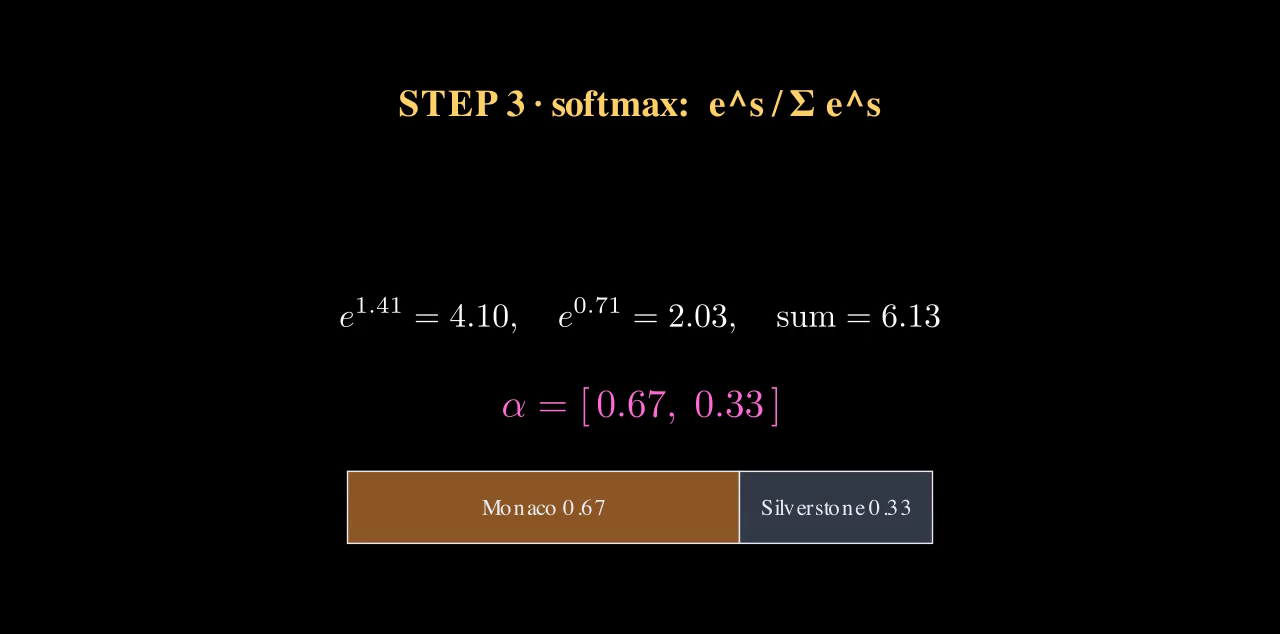
Step 4, blend: 0.67·[2,1] + 0.33·[1,2] = [1.67, 1.33] = m₁ Step 5, eq 7: sum the routes and add the self-term ONCE: m₁ = [1.67, 1.33] races → standings m₂ = [1.5, 0.5 ] races → results m₃ = [0.5, 1.0 ] constructors → results self = [1, 0] h_Hamilton = [1,0] + [1.67,1.33] + [1.5,0.5] + [0.5,1.0] = [4.67, 2.83]
Note that the self-term is added once, at the end, not stirred into every route message, or Hamilton gets counted three times over. That's a detail I got wrong the first time through.
![Hamilton goes from [1, 0] to [4.67, 2.83].](../assets/relgnn/13-walk-final.png)
The scoreboard
The test is RelBench: seven real relational databases, thirty prediction tasks, three flavours: classification (ROC-AUC, higher better), regression (mean absolute error, lower better), and recommendation (mean average precision, higher better). Split by time, train on the past, test on the future: the leakage rule from chapter one. The baseline that matters is a heterogeneous graph network: the two-hop crawler this whole piece has been fixing.
Before looking, predict: RelGNN's advantage is handling bridges and hubs, so where should it win biggest: databases full of tangled junction tables, or simple ones that are basically a chain?
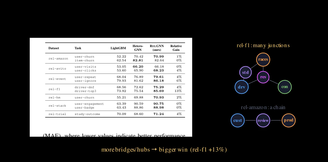
On regression, the headline of the paper: on the clinical-trial database, predicting a site's success rate, error drops from 0.400 to 0.301, a 25% improvement. On recommendation, RelGNN is better than or equal to the baseline on every single task. Totalled up: state of the art on 27 of 30 tasks, more than 4% better on 17 of them, up to +25%.
The ablation, which is the real story
Now the bet. To settle it the authors build a crippled RelGNN: keep the atomic routes, rip out the attention, replace it with the same dumb averaging the baseline uses. If attention is the engine, this version should collapse.
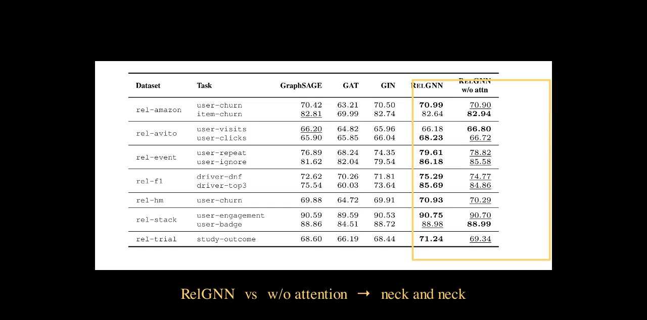
The gains come from the atomic routes, not the attention. From fixing the plumbing so the right nodes talk in one clean hop. The attention just decides how loudly. And the routes hold up whichever graph network you drop them into: GraphSAGE, GAT, GIN.
If I remember one thing from this paper, it's that: it wasn't a fancier aggregator that won. It was respecting the structure of the database.
Two honest cracks
On one database, a question-and-answer network, RelGNN barely moves the needle, and the reason is telling. That database has a table whose rows link to other rows of the same table: posts linking to posts. Every route we built assumed a link joins two different tables, a source type and a destination type. When a table points at itself, source and destination are the same, and the neat bridge–hub picture blurs. The paper flags it as future work and sketches a fix worth about +2%.
And on the clinical-trial tasks the results wobble, likely the small scoring head bolted on the end that turns an embedding into a prediction, rather than the routes themselves.
Could you have invented it?
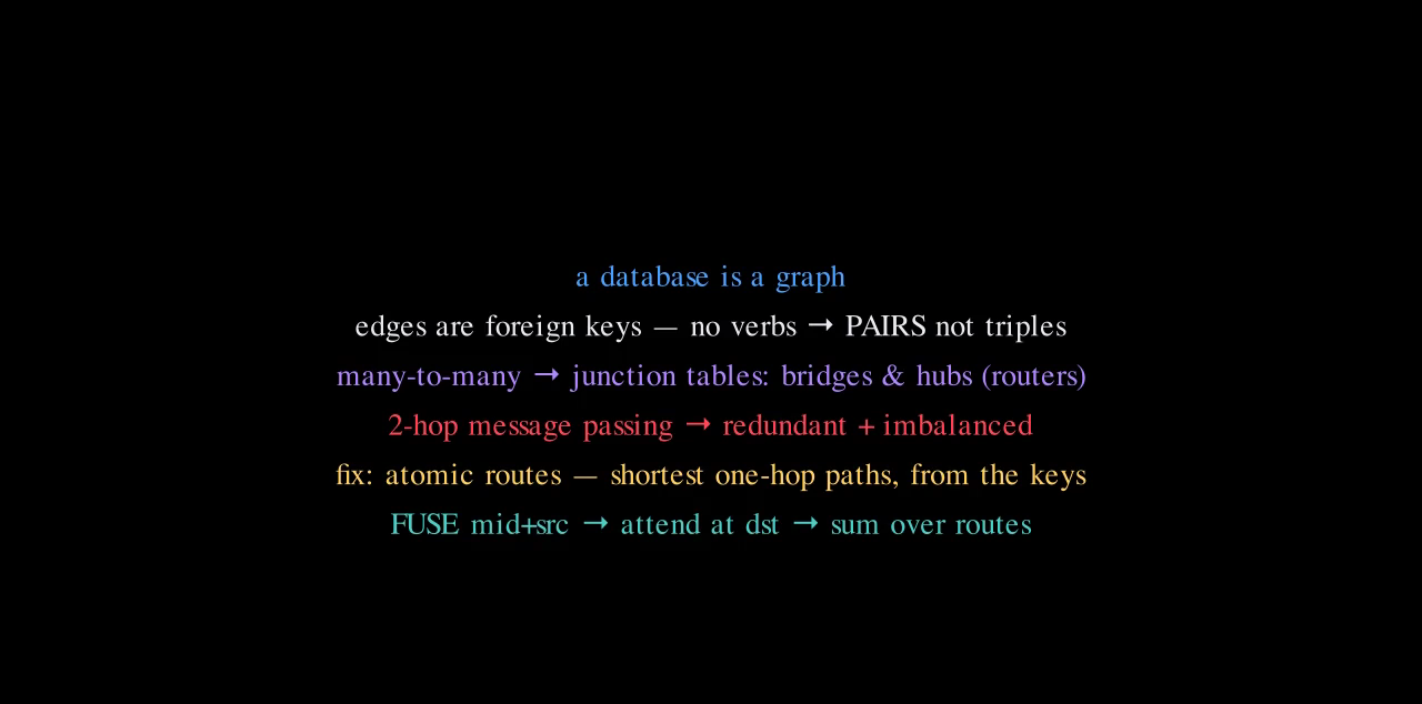
A database is a graph. Its edges are only foreign keys, no verbs, so the unit is a pair, not a triple. Many-to-many forces junction tables: bridges and hubs, routers carrying all the traffic. Standard message passing crawls two hops through them and comes out redundant and imbalanced. Fix it with atomic routes: the shortest one-hop paths, read straight off the keys. Fuse the middle with the source, aggregate at the destination, sum over routes with separate weights. That's the whole paper.
Capstone
Take a database you actually know: your company's, a game's, anything with a few linked tables.
- Draw its schema and mark every bridge and hub.
- List its atomic routes straight off the foreign keys.
- Pick one node and write the shape of a single composite update for it: fuse, attend, sum.
If you can do that, you don't just understand this paper; you can teach it.
Paper: RelGNN: Composite Message Passing for Relational Deep Learning, Chen et al., ICML 2025. Figures are stills I built while working through it. Corrections very welcome: surajprasad8977@gmail.com.